Fluid Mechanics Course
The Navier-Stokes Equations
Lecturer: Jacob Andersen
Slides by Asst. Prof. Jacob Andersen (AAU BUILD) and Assoc. Prof. Jakob Hærvig (AAU ENERGY)
Introduction to the Navier-Stokes Equations
Any experience with the Navier-Stokes Equations?
What are they?
Popularly: Very general set of equations describing almost any flow of fluids
- Vast span of applications
What makes them special?
- Recall: Potential flow theory
- Inviscid, irrotational, incompressible flow
- The most general form of the Navier-Stokes equations
- Viscid, rotational, compressible flow
- Huge impact on the complexity of the flow → Turbulence
Flow over stalled airfoil
- Note: Incompressibility is still a very accurate assumption used in most engineering applications
Richard Feynman on Turbulence
Turbulence is the most important unsolved problem of classical physics
Eames & Flor (2011)
There is a physical problem that is common to many fields, that is very old, and that has not been solved. It is not the problem of finding new fundamental particles, but something left over from a long time ago—over a hundred years. Nobody in physics has really been able to analyze it mathematically satisfactorily in spite of its importance to the sister sciences. It is the analysis of circulating or turbulent fluids.
Feynman et al. (1965)
A Millennium Problem
The Clay Mathematics Institute has identified the existence and smoothness of solutions to the Navier-Stokes equations as one of the seven Millennium Prize Problems.
-
Sketch of the Problem
Prove or give a counter-example that in 3-D, solutions to the incompressible Navier-Stokes equations always exist and are smooth for all time.
Fefferman (2022) -
Prize
$1,000,000 for a correct solution.
We Are Engineers - Why This Lecture?
The Navier-Stokes equations describes some very complex physics not fully understood and their mathematical properties are still being investigated by mathematicians
- This is a course for engineering programmes
- We need to able to reach results and within a reasonable time frame
- So, why this lecture?
- Combined with modern computer power the Navier-Stokes equations
- Allows for detailed analysis of virtually all flows of engineering interest
- Are great for investigation of novel concepts — given their generality
- Are often the basis of faster, more simple design frameworks
- Understanding the underlying physics of the Navier-Stokes equations is key to applying them meaningfully
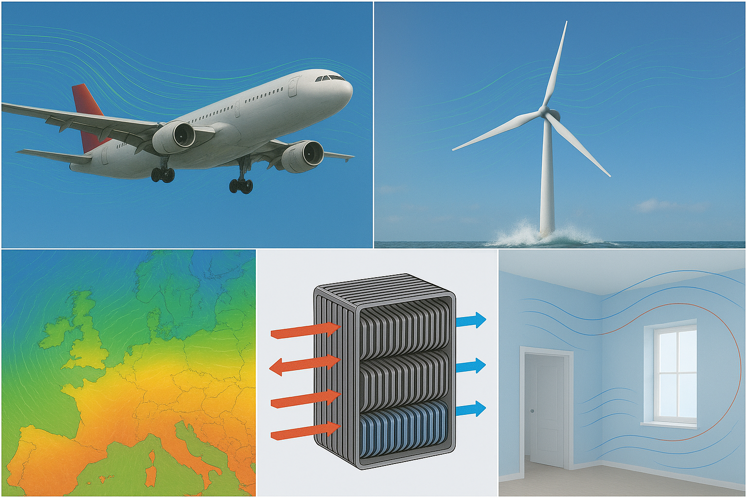
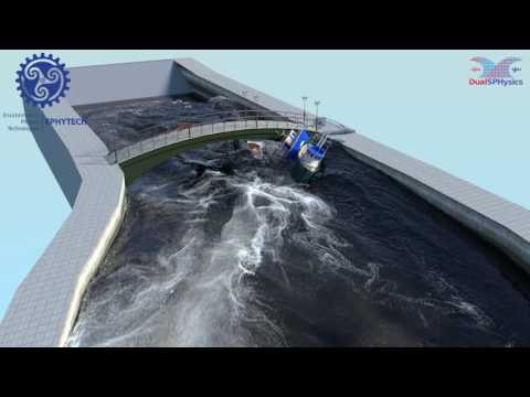
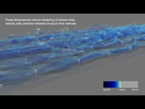
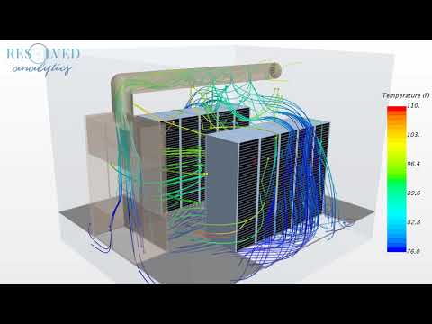
Engineering Applications
Examples of Engineering Applications based on Navier-Stokes solvers (CFD):

Learning Goals
Learning Goals
Knowledge
- Must have knowledge about stresses in fluids, equation of motion, constitutive models and Navier-Stokes equations.
Skills
- Must be able to describe assumptions and limitations of mathematical models for different types of flows.
- Must be able to apply analytical and semi-empirical methods for mathematical description of fluid dynamic problems.
Differential Analysis
Differential Analysis
Objective: Detailed information on flow inside domain of interest
- Local values of flow fields (velocity, pressure, etc.) not obtained with integral methods
- Finite → Infinitesimal control volume (CV)
- Governing equations: Partial differential equations (PDEs) derived from conservation laws on
- Mass
- Linear momentum
Fluid Element Kinematics
Fluid Element Kinematics
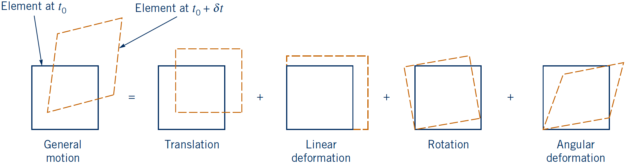
- System approach (rather than CV approach)
- Development of kinematic relations for infinitesimal system (fluid element)
Translation
- Velocity gradients are zero
- Pure translation: No deformation
- Rigid body motion of fluid element
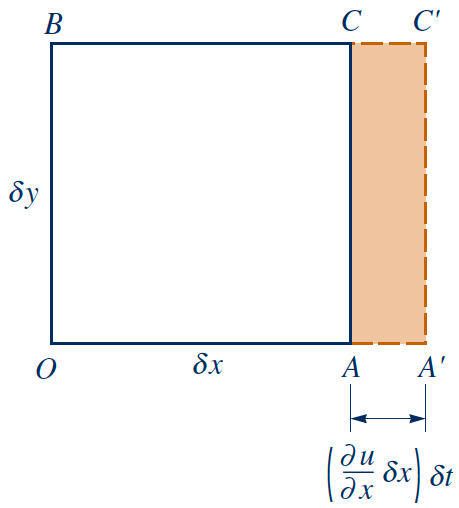
Linear deformation
- Non-zero velocity gradient in 1-D: $\frac{\partial u}{\partial x} \neq 0$
- Stretching/compression of fluid element
- Change of length of line $OA$ per $\delta t$: Linear strain rate $$\dot{\epsilon}_{xx}=\frac{\partial u}{\partial x} ~~~\text{(1-D)}$$
- Rate of change of volume per unit volume: Volumetric dilatation rate $$\frac{\partial u}{\partial x} + \frac{\partial v}{\partial y} + \frac{\partial w}{\partial z} = \boldsymbol{\nabla} \cdot \boldsymbol{V} ~~~\text{(3-D)}$$
- Incompressibility?
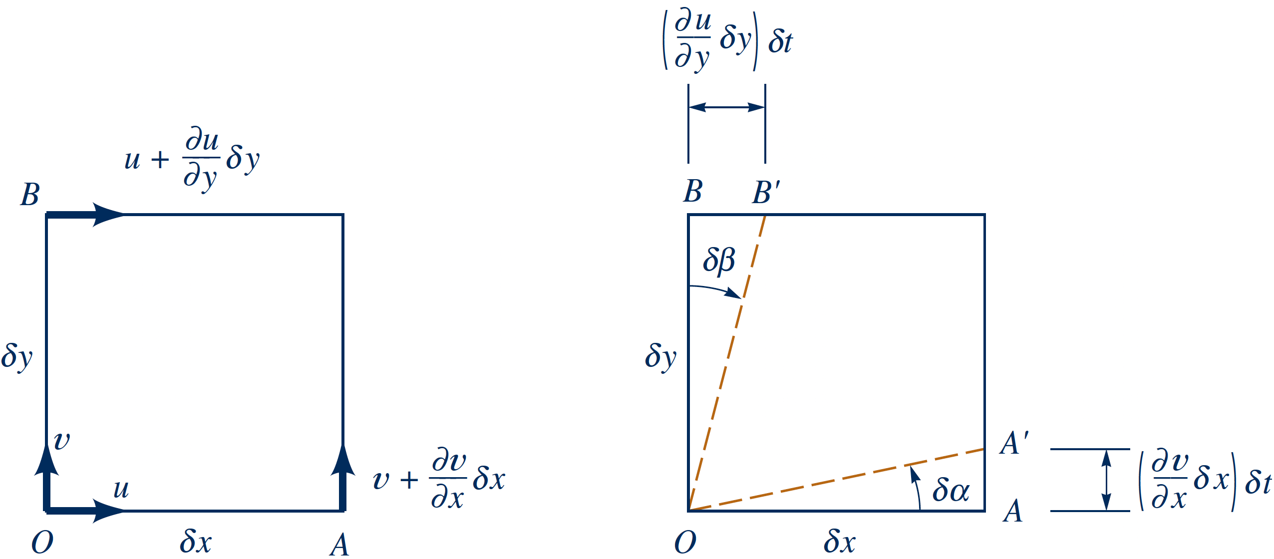
Rotation
- Cross derivatives $\frac{\partial u}{\partial y} \neq 0$ and $\frac{\partial v}{\partial x} \neq 0$
- Line $OA$ rotates with $\delta \alpha = -\delta \beta$ in $\delta t$ (rigid body rotation)
- Assuming small angles $$\tan(\delta \alpha)=\delta \alpha=\frac{AA'}{\delta x}=\frac{\partial v}{\partial x}\delta t$$
- Angular velocity: $$\omega_{OA}=\lim_{\delta t \to 0}\frac{\delta \alpha}{\delta t}=\frac{\partial v}{\partial x}$$ $$\omega_{OB}=\lim_{\delta t \to 0}\frac{\delta \beta}{\delta t}=\frac{\partial u}{\partial y}$$
Rotation
- Angular velocity: $\omega_{OA}=\frac{\partial v}{\partial x}$ and $\omega_{OB}=\frac{\partial u}{\partial y}$
- Average rate of rotation of element about $z$ (counter-clockwise is positive) $$\omega_z=\frac{1}{2}\left(\frac{\partial v}{\partial x}-\frac{\partial u}{\partial y}\right)$$
- Similarly for rotation about $x$ and $y$ axes. In 3-D, $$\boldsymbol{\omega}=\frac{1}{2}\boldsymbol{\nabla} \times \boldsymbol{V}$$
- Which is related to vorticity as $\boldsymbol{\zeta} = 2\boldsymbol{\omega}$
- $\boldsymbol{\zeta}$ in irrotational flow?
Angular deformation
- $\omega_{OA} \neq -\omega_{OB}$
- Change of shape of fluid element
- Change of the angle between $OA$ and $OB$: Shearing strain $$\delta \gamma_{xy}=\delta \alpha + \delta \beta$$
- Rate of change of shearing strain: Shear strain rate
$$\dot{\gamma}_{xy}=\lim_{\delta t \to 0}\frac{\delta \gamma_{xy}}{\delta t}=\frac{\partial v}{\partial x}+\frac{\partial u}{\partial y}$$
- Important measure for viscous stresses in fluids
Derivation of the Continuity Equation
Derivation of the Continuity Equation
Conservation of mass for a finite CV (application of Reynolds Transport Theorem) $$\frac{D M_{sys}}{D t} = \frac{d}{dt}\int_{CV} \rho \, dV\llap{--} + \int_{CS} \rho \boldsymbol{V} \cdot \boldsymbol{\hat{n}} \, dA = 0$$
- Goal: Conservation of mass for a infinitesimal CV
Derivation of the Continuity Equation
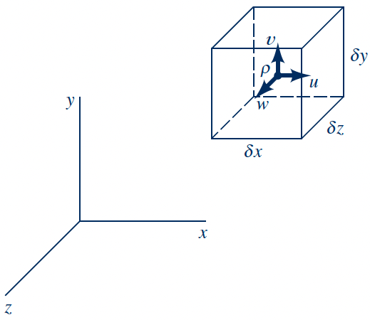
Consider an infinitesimal control volume with dimensions $\delta x\,\delta y\,\delta z$
- Fields given in centroid: $\rho, \boldsymbol{V}$
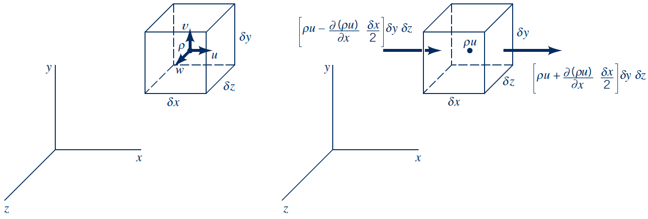
Infinitesimal CV with mass flow rate in $x$ at faces
Derivation of the Continuity Equation
Reformulation of volume integral and surface integrals $$ \frac{D M_{sys}}{D t} = \textcolor{#cc445b}{\frac{d}{dt}\int_{CV} \rho \, dV\llap{--}} + \textcolor{#0e8563}{\int_{CS} \rho \boldsymbol{V} \cdot \boldsymbol{\hat{n}} \, dA} = 0 $$
Infinitesimal CV with mass flow rate in $x$ at faces
- Approximation of volume integral for infinitesimal CV, $$ \textcolor{#cc445b}{\frac{d}{dt}\int_{CV} \rho \, dV\llap{--}} \approx \frac{\partial \rho}{\partial t} \, \delta x\, \delta y\, \delta z $$
Derivation of the Continuity Equation
Reformulation of surface integral $$ \frac{D M_{sys}}{D t} = \frac{\partial \rho}{\partial t} \, \delta x\, \delta y\, \delta z + \textcolor{#0e8563}{\int_{CS} \rho \boldsymbol{V} \cdot \boldsymbol{\hat{n}} \, dA} = 0 $$
Infinitesimal CV with mass flow rate in $x$ at faces
- Mass flux (rate of mass flow per unit area) in $x$ at centroid: $\rho u$
- Mass flux at faces (First order Taylor series expansion): $$\rho u |_{x+\delta x /2} = \rho u + \frac{\partial (\rho u)}{\partial x} \frac{\delta x}{2}$$ $$\rho u |_{x-\delta x /2} = \rho u - \frac{\partial (\rho u)}{\partial x} \frac{\delta x}{2}$$
Derivation of the Continuity Equation
Reformulation of surface integral $$ \frac{D M_{sys}}{D t} = \frac{\partial \rho}{\partial t} \, \delta x\, \delta y\, \delta z + \textcolor{#0e8563}{\int_{CS} \rho \boldsymbol{V} \cdot \boldsymbol{\hat{n}} \, dA} = 0 $$
- Mass flux (mass flow rate per unit area) in $x$ at centroid: $\rho u$
- Mass flux in $x$ at faces (First order Taylor series expansion): $$\rho u |_{x+\delta x /2} = \rho u + \frac{\partial (\rho u)}{\partial x} \frac{\delta x}{2}$$ $$\rho u |_{x-\delta x /2} = \rho u - \frac{\partial (\rho u)}{\partial x} \frac{\delta x}{2}$$
- Net mass flow rate in $x$: $$(\rho u |_{x+\delta x /2} - \rho u |_{x-\delta x /2}) \, \delta y\, \delta z \textcolor{#FFFFFF}{= \frac{\partial (\rho u)}{\partial x} \, \delta x\, \delta y\, \delta z}$$
Derivation of the Continuity Equation
Reformulation of surface integral $$ \frac{D M_{sys}}{D t} = \frac{\partial \rho}{\partial t} \, \delta x\, \delta y\, \delta z + \textcolor{#0e8563}{\int_{CS} \rho \boldsymbol{V} \cdot \boldsymbol{\hat{n}} \, dA} = 0 $$
- Mass flux (mass flow rate per unit area) in $x$ at centroid: $\rho u$
- Mass flux in $x$ at faces (First order Taylor series expansion): $$\rho u |_{x+\delta x /2} = \cancel{\rho u} + \frac{\partial (\rho u)}{\partial x} \frac{\delta x}{\cancel{2}}$$ $$\rho u |_{x-\delta x /2} = \cancel{\rho u} - \frac{\partial (\rho u)}{\partial x} \frac{\delta x}{\cancel{2}}$$
- Net mass flow rate in $x$: $$(\rho u |_{x+\delta x /2} - \rho u |_{x-\delta x /2}) \, \delta y\, \delta z = \frac{\partial (\rho u)}{\partial x} \, \delta x\, \delta y\, \delta z$$
- Similarly for net mass flow rate in $y$ and $z$ directions: $$\frac{\partial (\rho v)}{\partial y} \, \delta x\, \delta y\, \delta z \ \ \text{and} \ \ \frac{\partial (\rho w)}{\partial z} \, \delta x\, \delta y\, \delta z$$
- Net mass flow rate (3-D): $$\textcolor{#0e8563}{\int_{CS} \rho \boldsymbol{V} \cdot \boldsymbol{\hat{n}} \, dA} = \left(\frac{\partial (\rho u)}{\partial x} + \frac{\partial (\rho v)}{\partial y} + \frac{\partial (\rho w)}{\partial z}\right) \, \delta x\, \delta y\, \delta z $$
Derivation of the Continuity Equation
Reformulation of surface integral $$ \frac{D M_{sys}}{D t} = \frac{\partial \rho}{\partial t} \, \delta x\, \delta y\, \delta z + \textcolor{#0e8563}{\int_{CS} \rho \boldsymbol{V} \cdot \boldsymbol{\hat{n}} \, dA} = 0 $$
- Mass flux (mass flow rate per unit area) in $x$ at centroid: $\rho u$
- Mass flux in $x$ at faces (First order Taylor series expansion): $$\rho u |_{x+\delta x /2} = \cancel{\rho u} + \frac{\partial (\rho u)}{\partial x} \frac{\delta x}{\cancel{2}}$$ $$\rho u |_{x-\delta x /2} = \cancel{\rho u} - \frac{\partial (\rho u)}{\partial x} \frac{\delta x}{\cancel{2}}$$
- Net mass flow rate in $x$: $$(\rho u |_{x+\delta x /2} - \rho u |_{x-\delta x /2}) \, \delta y\, \delta z = \frac{\partial (\rho u)}{\partial x} \, \delta x\, \delta y\, \delta z$$
- Similarly for net mass flow rate in $y$ and $z$ directions: $$\frac{\partial (\rho v)}{\partial y} \, \delta x\, \delta y\, \delta z \ \ \text{and} \ \ \frac{\partial (\rho w)}{\partial z} \, \delta x\, \delta y\, \delta z$$
- Net mass flow rate (3-D): $$\textcolor{#0e8563}{\int_{CS} \rho \boldsymbol{V} \cdot \boldsymbol{\hat{n}} \, dA} = \nabla \cdot (\rho \boldsymbol{V}) \, \delta x\, \delta y\, \delta z$$
Derivation of the Continuity Equation
Reformulation $$ \frac{D M_{sys}}{D t} = \frac{\partial \rho}{\partial t} \, \delta x\, \delta y\, \delta z + \nabla \cdot (\rho \boldsymbol{V}) \, \delta x\, \delta y\, \delta z = 0$$
$$ \Downarrow $$ $$ \left( \frac{\partial \rho}{\partial t} + \nabla \cdot (\rho \boldsymbol{V}) \right) \delta x\, \delta y\, \delta z = 0 $$The compressible continuity equation:
$$\frac{\partial \rho}{\partial t} + \nabla \cdot (\rho \boldsymbol{V}) = 0$$Incompressibility?
Derivation of the Continuity Equation
Reformulation $$ \frac{D M_{sys}}{D t} = \frac{\partial \rho}{\partial t} \, \delta x\, \delta y\, \delta z + \nabla \cdot (\rho \boldsymbol{V}) \, \delta x\, \delta y\, \delta z = 0$$
$$ \Downarrow $$ $$ \left( \frac{\partial \rho}{\partial t} + \nabla \cdot (\rho \boldsymbol{V}) \right) \delta x\, \delta y\, \delta z = 0 $$The compressible continuity equation:
$$\frac{\partial \rho}{\partial t} + \nabla \cdot (\rho \boldsymbol{V}) = 0$$The incompressible continuity equation:
$$\nabla \cdot \boldsymbol{V} = 0$$Corresponds to a zero volumetric dilatation rate
Derivation of the Navier-Stokes Equations
Derivation of the Navier-Stokes Equations
Approach
- Conservation of linear momentum for an infinitesimal CV
- Forces acting on an infinitesimal CV
- Equations of fluid motion
- Constitutive law for Newtonian fluids
- The Navier-Stokes equations
Derivation of the Navier-Stokes Equations
Conservation of linear momentum for a finite CV (application of Reynolds Transport Theorem) $$ \boldsymbol{F} = \frac{D \boldsymbol{P_{sys}}}{D t} = \frac{d}{dt}\int_{CV} \boldsymbol{V} \rho \, dV\llap{--} + \int_{CS} \boldsymbol{V}\rho \boldsymbol{V} \cdot \boldsymbol{\hat{n}} \, dA$$
- Similar methodology as used to derive the continuity equation: Reformulation to an infinitesimal CV
Derivation of the Navier-Stokes Equations
Conservation of linear momentum for a finite CV (application of Reynolds Transport Theorem)
$$\boldsymbol{F} = \frac{D \boldsymbol{P_{sys}}}{D t} =
\textcolor{#cc445b}{\frac{d}{dt}\int_{CV} \boldsymbol{V}\rho \, dV\llap{--}}
+
\textcolor{#0e8563}{\int_{CS} \boldsymbol{V}\rho \boldsymbol{V} \cdot \boldsymbol{\hat{n}} \, dA}
$$
Infinitesimal CV
Derivation of the Navier-Stokes Equations
Conservation of linear momentum $$ \boldsymbol{F} = \frac{D \boldsymbol{P_{sys}}}{D t} = \frac{\partial}{\partial t} (\rho \boldsymbol{V}) \, \delta x\, \delta y\, \delta z + \textcolor{#0e8563}{\int_{CS} \boldsymbol{V}\rho \boldsymbol{V} \cdot \boldsymbol{\hat{n}} \, dA} $$
- Similar methodology as used to derive the continuity equation: Reformulation to an infinitesimal CV
- We reuse a result from 3-D mass conservation: Net mass flow rate → net linear momentum flow rate $$\text{Mass cons.:} \ \ \textcolor{#0e8563}{\int_{CS} \rho \boldsymbol{V} \cdot \boldsymbol{\hat{n}} \, dA} = \left(\frac{\partial (\rho u)}{\partial x} + \frac{\partial (\rho v)}{\partial y} + \frac{\partial (\rho w)}{\partial z}\right) \, \delta x\, \delta y\, \delta z = \nabla \cdot (\rho \boldsymbol{V}) \, \delta x\, \delta y\, \delta z $$ $$\text{Momentum cons.:} \ \ \textcolor{#0e8563}{\int_{CS} \boldsymbol{V}\rho \boldsymbol{V} \cdot \boldsymbol{\hat{n}} \, dA} = \left(\frac{\partial (\rho u\boldsymbol{V})}{\partial x} + \frac{\partial (\rho v\boldsymbol{V})}{\partial y} + \frac{\partial (\rho w\boldsymbol{V})}{\partial z}\right) \, \delta x\, \delta y\, \delta z = \nabla \cdot (\rho\boldsymbol{V}\boldsymbol{V}) \, \delta x\, \delta y\, \delta z $$
Derivation of the Navier-Stokes Equations
Conservation of linear momentum for infinitesimal CV $$ \delta \boldsymbol{F} = \frac{\partial}{\partial t} (\rho \boldsymbol{V}) \, \delta x\, \delta y\, \delta z + \nabla \cdot (\rho\boldsymbol{V}\boldsymbol{V}) \, \delta x\, \delta y\, \delta z $$ $$ \Updownarrow $$ $$ \delta \boldsymbol{F} = \left( \frac{\partial}{\partial t} (\rho \boldsymbol{V}) + \nabla \cdot (\rho \boldsymbol{V}\boldsymbol{V}) \right) \, \delta x\, \delta y\, \delta z $$
- Application of Leibniz product rule on first term: $$\frac{\partial}{\partial t} (\rho \boldsymbol{V}) = \rho \frac{\partial \boldsymbol{V}}{\partial t} + \boldsymbol{V} \frac{\partial \rho}{\partial t}$$
- Application of Leibniz product rule on second term (divergence of a dyad/outer product of two vectors): $$\nabla \cdot (\rho \boldsymbol{V}\boldsymbol{V}) = \rho (\boldsymbol{V} \cdot \nabla) \boldsymbol{V} + \boldsymbol{V} (\nabla \cdot (\rho \boldsymbol{V}))$$
- Insertion and rearrangement $$ \delta \boldsymbol{F} = \left( \rho \left( \frac{\partial \boldsymbol{V}}{\partial t} + (\boldsymbol{V} \cdot \nabla) \boldsymbol{V} \right) + \boldsymbol{V} \left( \frac{\partial \rho}{\partial t} + \nabla \cdot (\rho \boldsymbol{V})\right) \right) \, \delta x\, \delta y\, \delta z \textcolor{#cc445b00}{= \rho \left( \frac{D \boldsymbol{V}}{D t} \right) \, \delta x\, \delta y\, \delta z} $$
Derivation of the Navier-Stokes Equations
Conservation of linear momentum for infinitesimal CV $$ \delta \boldsymbol{F} = \frac{\partial}{\partial t} (\rho \boldsymbol{V}) \, \delta x\, \delta y\, \delta z + \nabla \cdot (\rho\boldsymbol{V}\boldsymbol{V}) \, \delta x\, \delta y\, \delta z $$ $$ \Updownarrow $$ $$ \delta \boldsymbol{F} = \left( \frac{\partial}{\partial t} (\rho \boldsymbol{V}) + \nabla \cdot (\rho \boldsymbol{V}\boldsymbol{V}) \right) \, \delta x\, \delta y\, \delta z $$
- Application of Leibniz product rule on first term: $$\frac{\partial}{\partial t} (\rho \boldsymbol{V}) = \rho \frac{\partial \boldsymbol{V}}{\partial t} + \boldsymbol{V} \frac{\partial \rho}{\partial t}$$
- Application of Leibniz product rule on second term (divergence of a dyad/outer product of two vectors): $$\nabla \cdot (\rho \boldsymbol{V}\boldsymbol{V}) = \rho (\boldsymbol{V} \cdot \nabla) \boldsymbol{V} + \boldsymbol{V} (\nabla \cdot (\rho \boldsymbol{V}))$$
- Applying the material derivative and the (compressible) continuity equation $$ \delta \boldsymbol{F} = \left( \rho \left( \textcolor{#cc445b}{\frac{\partial \boldsymbol{V}}{\partial t} + (\boldsymbol{V} \cdot \nabla) \boldsymbol{V}} \right) + \textcolor{#31a9c1}{\cancel{ \boldsymbol{V} \left( \frac{\partial \rho}{\partial t} + \nabla \cdot (\rho \boldsymbol{V})\right) }} \right) \, \delta x\, \delta y\, \delta z = \rho \left( \frac{D \boldsymbol{V}}{D t} \right) \, \delta x\, \delta y\, \delta z$$
- Conservation of linear momentum on infinitesimal CV $\rightarrow$ differential form of Newton's 2nd law $$ \delta \boldsymbol{F} = \delta m \ \boldsymbol{a} $$
Derivation of the Navier-Stokes Equations
Next step: Describe the forces $\delta \boldsymbol{F}$ acting on the infinitesimal CV
- Combination of body forces (e.g., gravity) and surface forces
(e.g. pressure, viscous stresses) $$ \delta \boldsymbol{F} = \textcolor{#cc445b}{\delta \boldsymbol{F_{b}}} + \textcolor{#0e8563}{\delta \boldsymbol{F_{s}}} $$ - Body force due to gravity (3-D): $$ \textcolor{#cc445b}{\delta \boldsymbol{F_{b}}} = \delta m \ \boldsymbol{g} $$
Derivation of the Navier-Stokes Equations
Next step: Describe the forces $\delta \boldsymbol{F}$ acting on the infinitesimal CV
- Combination of body forces (e.g., gravity) and surface forces
(e.g. pressure, viscous stresses) $$ \delta \boldsymbol{F} = \delta m \ \boldsymbol{g} + \textcolor{#0e8563}{\delta \boldsymbol{F_{s}}} $$ - Surface force: A combination of normal and shear stresses
- Stress expected to vary in flow field
- First order Taylor series expansion on stress state
(incl. gradients) in centroid - Net surface force in $x$ direction $$ \delta \boldsymbol{F_{sx}} = \left( \frac{\partial \sigma_{xx}}{\partial x} + \frac{\partial \tau_{yx}}{\partial y} + \frac{\partial \tau_{zx}}{\partial z} \right) \ \delta x\ \delta y\ \delta z $$
- Similarly for $y$ and $z$ directions
- Introducing Cauchy's stress tensor $\boldsymbol{\sigma}$ $$ \boldsymbol{\sigma} = \begin{bmatrix} \sigma_{xx} & \tau_{xy} & \tau_{xz} \\ \tau_{yx} & \sigma_{yy} & \tau_{yz} \\ \tau_{zx} & \tau_{zy} & \sigma_{zz} \end{bmatrix} $$
- The net surface force vector can be expressed as $$ \textcolor{#0e8563}{\delta \boldsymbol{F_{s}}}= \left( \nabla \cdot \boldsymbol{\sigma} \right) \, \delta x\, \delta y\, \delta z $$

Infinitesimal CV with surfaces forces acting in $x$
Derivation of the Navier-Stokes Equations
Description of the net force $\delta \boldsymbol{F}$ acting on the infinitesimal CV
- Combination of body forces (e.g., gravity) and surface forces
(e.g. pressure, viscous stresses) $$ \delta \boldsymbol{F} = \delta m \ \boldsymbol{g} + ( \nabla \cdot \boldsymbol{\sigma} ) \, \delta x\, \delta y\, \delta z $$
$$ \Updownarrow $$
$$ \ \delta \boldsymbol{F} = ( \rho \ \boldsymbol{g} + ( \nabla \cdot \boldsymbol{\sigma} )) \, \delta x\, \delta y\, \delta z $$
- We recall $$ \delta \boldsymbol{F} = \delta m \ \boldsymbol{a} $$ $$ \Downarrow $$ $$ ( \rho \ \boldsymbol{g} + ( \nabla \cdot \boldsymbol{\sigma} )) \, \delta x\, \delta y\, \delta z = \rho \left( \frac{D \boldsymbol{V}}{D t} \right)\, \delta x\, \delta y\, \delta z $$
Derivation of the Navier-Stokes Equations
Description of the net force $\delta \boldsymbol{F}$ acting on the infinitesimal CV
- Combination of body forces (e.g., gravity) and surface forces
(e.g. pressure, viscous stresses) $$ \delta \boldsymbol{F} = \delta m \ \boldsymbol{g} + ( \nabla \cdot \boldsymbol{\sigma} ) \, \delta x\, \delta y\, \delta z $$
$$ \Updownarrow $$
$$ \ \delta \boldsymbol{F} = ( \rho \ \boldsymbol{g} + ( \nabla \cdot \boldsymbol{\sigma} )) \, \delta x\, \delta y\, \delta z $$
- We recall $$ \delta \boldsymbol{F} = \delta m \ \boldsymbol{a} $$ $$ \Downarrow $$ $$ ( \rho \ \boldsymbol{g} + ( \nabla \cdot \boldsymbol{\sigma} )) \, \cancel{\delta x\, \delta y\, \delta z} = \rho \left( \frac{D \boldsymbol{V}}{D t} \right) \, \cancel{\delta x\, \delta y\, \delta z} $$
- The general differential equations of fluid motion,
or the Cauchy momentum equation, results $$ \rho \ \boldsymbol{g} + ( \nabla \cdot \boldsymbol{\sigma} ) = \rho \left( \frac{\partial \boldsymbol{V}}{\partial t} + (\boldsymbol{V} \cdot \nabla) \boldsymbol{V} \right) $$
Derivation of the Navier-Stokes Equations
Key result: The general differential equations of fluid motion (Cauchy momentum equation): $$ \rho \ \boldsymbol{g} + ( \nabla \cdot \boldsymbol{\sigma} ) = \rho \left( \frac{\partial \boldsymbol{V}}{\partial t} + (\boldsymbol{V} \cdot \nabla) \boldsymbol{V} \right) $$
- Resemblance to $\delta \boldsymbol{F} = \delta m \ \boldsymbol{a}$
- Written out the equations of fluid motion reads: $$ \rho g_x + \frac{\partial \sigma_{xx}}{\partial x} + \frac{\partial \tau_{yx}}{\partial y} + \frac{\partial \tau_{zx}}{\partial z} = \rho \left( \frac{\partial u}{\partial t} + u\frac{\partial u}{\partial x} + v\frac{\partial u}{\partial y} + w\frac{\partial u}{\partial z} \right) $$ $$ \rho g_y + \frac{\partial \tau_{xy}}{\partial x} + \frac{\partial \sigma_{yy}}{\partial y} + \frac{\partial \tau_{zy}}{\partial z} = \rho \left( \frac{\partial v}{\partial t} + u\frac{\partial v}{\partial x} + v\frac{\partial v}{\partial y} + w\frac{\partial v}{\partial z} \right) $$ $$ \rho g_z + \frac{\partial \tau_{xz}}{\partial x} + \frac{\partial \tau_{yz}}{\partial y} + \frac{\partial \sigma_{zz}}{\partial z} = \rho \left( \frac{\partial w}{\partial t} + u\frac{\partial w}{\partial x} + v\frac{\partial w}{\partial y} + w\frac{\partial w}{\partial z} \right) $$
- Can we solve the flow field now?
- No, more unknowns (6 stress components, 3 velocity components, pressure and density) than equations → Ill-posed problem
Derivation of the Navier-Stokes Equations
To close the problem, we need to relate stresses to velocities, i.e., elimate unkowns
- Revisit the Cauchy stress tensor: Sum of pressure (isotropic) and viscous (deviatoric) stress tensors $$\boldsymbol{\sigma} = -p \boldsymbol{I_3} + \boldsymbol{\tau} = \begin{bmatrix} -p & 0 & 0 \\ 0 & -p & 0 \\ 0 & 0 & -p \end{bmatrix} + \begin{bmatrix} \tau_{xx} & \tau_{xy} & \tau_{xz} \\ \tau_{yx} & \tau_{yy} & \tau_{yz} \\ \tau_{zx} & \tau_{zy} & \tau_{zz} \end{bmatrix} $$
- Constitutive relation for an incompressible Newtonian fluid: Viscous stresses are linearly proportional to strain rates $$\boldsymbol{\tau} = \mu \boldsymbol{S} $$
- with the strain rate tensor $$ \boldsymbol{S} = \left[ \begin{matrix} 2 \dot{\epsilon}_{xx} & \dot{\gamma}_{xy} & \dot{\gamma}_{xz} \\ \dot{\gamma}_{yx} & 2 \dot{\epsilon}_{yy} & \dot{\gamma}_{yz} \\ \dot{\gamma}_{zx} & \dot{\gamma}_{zy} & 2 \dot{\epsilon}_{zz} \end{matrix} \right] $$
- Recalling our kinematic relations developed with the fluid element
- Strain rates were expressed in terms of velocity gradients $$ \boldsymbol{S} = \nabla \boldsymbol{V} + (\nabla \boldsymbol{V})^{\mathrm{T}} = \left[ \begin{matrix} 2\frac{\partial u}{\partial x} & \left(\frac{\partial u}{\partial y} + \frac{\partial v}{\partial x}\right) & \ \left(\frac{\partial u}{\partial z} + \frac{\partial w}{\partial x}\right) \\ \left(\frac{\partial v}{\partial x} + \frac{\partial u}{\partial y}\right) & 2\frac{\partial v}{\partial y} & \left(\frac{\partial v}{\partial z} + \frac{\partial w}{\partial y}\right) \\ \left(\frac{\partial w}{\partial x} + \frac{\partial u}{\partial z}\right) & \left(\frac{\partial w}{\partial y} + \frac{\partial v}{\partial z}\right) & 2\frac{\partial w}{\partial z} \end{matrix} \right] $$
- Sum of diagonal entries is zero (traceless) due to continuity
Derivation of the Navier-Stokes Equations
Stress tensor for incompressible Newtonian fluid $$ \boldsymbol{\sigma} = -p \boldsymbol{I_3} + \mu (\nabla \boldsymbol{V} + (\nabla \boldsymbol{V})^{\mathrm{T}}) $$
Substituting into the equations of fluid motion $$ \rho \ \boldsymbol{g} + \nabla \cdot \boldsymbol{\sigma} = \rho \left( \frac{\partial \boldsymbol{V}}{\partial t} + (\boldsymbol{V} \cdot \nabla) \boldsymbol{V} \right) $$ $$ \Downarrow $$ $$ \rho \ \boldsymbol{g} + \nabla \cdot (-p \boldsymbol{I_3} + \mu (\nabla \boldsymbol{V} + (\nabla \boldsymbol{V})^{\mathrm{T}})) = \rho \left( \frac{\partial \boldsymbol{V}}{\partial t} + (\boldsymbol{V} \cdot \nabla) \boldsymbol{V} \right) $$
Using vector calculus identities and the continuity equation $$ \nabla \cdot (p \boldsymbol{I_3}) = \nabla p $$ $$ \nabla \cdot (\nabla \boldsymbol{V}) = \nabla^2 \boldsymbol{V} $$ $$ \nabla \cdot ((\nabla \boldsymbol{V})^{\mathrm{T}}) = \nabla(\nabla \cdot \boldsymbol{V}) = 0 \ \ \text{(continuity)} $$
Final form of the incompressible Navier-Stokes equations $$ \rho\left( \frac{\partial \boldsymbol{V}}{\partial t} + (\boldsymbol{V} \cdot \nabla) \boldsymbol{V} \right) = -\nabla p + \mu \nabla^2 \boldsymbol{V} + \rho \boldsymbol{g} $$
Derivation of the Navier-Stokes Equations
Final form of the incompressible Navier-Stokes equations $$ \rho\left( \frac{\partial \boldsymbol{V}}{\partial t} + (\boldsymbol{V} \cdot \nabla) \boldsymbol{V} \right) = -\nabla p + \rho \boldsymbol{g} + \mu \nabla^2 \boldsymbol{V} $$
- Together with the incompressible continuity equation, we have 4 equations for 4 unknowns ($u,v,w,p$) → well-posed problem!
- These are the governing equations of all incompressible Newtonian fluids!
- Now let's solve the equations!
Solving the Navier-Stokes Equations
Solving the Navier-Stokes Equations
We have now derived the formidable incompressible Navier-Stokes equations $$ \rho\left( \frac{\partial \boldsymbol{V}}{\partial t} + (\boldsymbol{V} \cdot \nabla) \boldsymbol{V} \right) = -\nabla p + \rho \boldsymbol{g} + \mu \nabla^2 \boldsymbol{V} $$
- What do we have here?
- A set of nonlinear 2nd order partial differential equations
- The nonlinear "self"-convection of momentum term $(\boldsymbol{V} \cdot \nabla) \boldsymbol{V}$
- Greatly complicates solutions
- Source of turbulence and instabilities
- Only few exact solutions and only for very simple flows
- No known accurate analytical solutions to most engineering flows
- Numerical methods for approximate solutions using CFD